The anatomy of search: In search of…

A galloping overview

As we have done before, let’s get a bird’s-eye view of the parts of the search process: text comes in and gets processed and stored in a database (called an index); a user submits a query; documents that match the query are retrieved from the index, ranked based on how well they match the query, and presented to the user.

Today we’ll look at the user’s query and how potential results are matched and ranked.

In search of…

At this point, we’ve done a lot of preparation getting our documents ready to be searched. In previous installments, we’ve looked at how we break text into tokens (which are approximately words, in English), normalize them (converting to lowercase, removing diacritics, and more), remove stop words, stem the remainder (converting them to their root forms), and store the results in an index (which is, roughly, a database of the words in all our documents). Now that we have our text stored in an index or two, things are going to move along much faster as we take advantage of all that preparation: we are ready for users to submit queries!

The first thing we do when we we get a user query is that we process it pretty much like we did the text we’ve indexed: we tokenize, normalize, and stem the query, so that the words of the query are in the same form as the words from our documents in our index.

Suppose a user—having unconsciously recast The Cat in the Hat in the mold of Of Mice and Men—searches for Of Cats and Hats.[1] Our tokens are Of, Cats, and, Hats. These get regularized—here just lowercased—to of, cats, and, hats. Removing stop words (of, and) and stemming the rest leaves cat, hat.

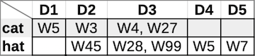
Looking up the two remaining words—cat and hat—in our index (which for now we’ll say has only five documents in it, D1–D5), we find the following document and word position information. (Note that “W4, W27” in column D3 for cat means that cat was found in Document #3 as Word #4 and #27):

Okay… what next?

AND and OR or NOT—Wait, what?

The classic search engine approach for combining search terms uses Boolean logic, which combines true and false values with AND, OR, and NOT operators.[2] In the search context, true and false refer to whether your search term is in a particular document. Basic search engines generally use an implicit AND operator. This means that a query like cat dog mouse is equivalent to cat AND dog AND mouse—requiring all three terms to be in a document for it to be shown as a result.

In our Of Cats and Hats example above, that means that both cat and hat need to be in a document for it to be shown as a result. We can see from the inverted index snippets above that both cat and hat occur in D2 and D3, while only cat is in D1 and only hat is in D4 and D5. So an implicit (or explicit[4]) AND operator would return the intersection of the two lists, namely D2 and D3 for the query Of Cats and Hats.

The OR operator returns the union of the two lists—so any document with either cat or hat is a good result. Thus, D1, D2, D3, D4, and D5 would all be results for cat OR hat.

Classic boolean search also allows you to exclude results that have a particular word in them, using NOT. So cat NOT hat would only return D1. (D2 and D3, while they do have cat in them, would be excluded because they also have some form of the now unwanted hat.)

As of August 2019, on-wiki search does not actually support boolean querying very well. By default, search behaves as if there were an implicit AND between query terms, and supports NOT for negation (you can use the NOT operator, or use a hyphen or an exclamation point). Parentheses are currently ignored, and explicit AND and OR are not well supported, especially when combined.[6]

Billions and Billions

If, as in our toy example above, you only get a handful of search results, their order doesn’t really matter all that much. But on English Wikipedia, for example, Of Cats and Hats gets over 15,000 results—with eight of the top ten all related to The Cat in the Hat. How did those results get to the top of the list?

We’ll again look at the classic search engine approach to this problem. Not all query terms are created equal: stop words are an explicit attempt to address the problem, but filtering them out causes its own problems. For example, “to be or not to be” is made up entirely of likely stop words, and there is a UK band called “The The”.[8] Stop words divide the world into black and white “useful” and “useless” categories, when reality calls for context-dependent shades of grey!

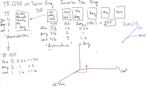
Enter term frequency (TF) and inverse document frequency (IDF), two extremely venerable measures of relevance in information retrieval. First, let’s recall our inverted index information for cat and hat that we have in our example index:

Term frequency is a measure of how many times a word appears in a given document. We see that cat appears in D1 and D2 only once, giving each a TF of 1, while it appears in D3 twice, giving a TF of 2. In some sense, then, D3 is arguably more “about” cats than D1 or D2.

Document frequency is a measure of how many different documents a word appears in. As we stipulated earlier, we have only five documents in our collection: D1–D5. We see that cat appears in 3/5 of all documents, while hat appears in 4/5. Inverse document frequency is the reciprocal of the document frequency (more or less, see below!)—so cat has an IDF of 1.67, while hat has an IDF of 1.25, making cat a slightly more valuable query term than hat.

The simplest version of a TF–IDF score for a word in a given document is just the TF value multiplied by the IDF value. You can then combine each document’s TF–IDF scores for all the words in your query to get a relevance score for each document, hopefully floating the best ones to the top of the results list.

Characteristic, yet distinctive

I like to say that term frequency measures how characteristic a word is of a document, while inverse document frequency is a measure of how distinctive a word is in a corpus—because TF and IDF are not absolute metrics for particular words, but depend heavily on context—i.e., on the corpus they find themselves in.

To see what we mean by “characteristic” and “distinctive”, consider the word the in a corpus of general English documents. It may appear hundreds of times in a given document (like this one!!), making it very characteristic of that document. On the other hand, it probably occurs in about 99% of English documents of reasonable length, so it is not very distinctive. In a multilingual collection of documents, though, with, say, only 5% of documents in English, the would probably be both characteristic and distinctive of English documents because it doesn’t appear in most non-English documents—unless the French are discussing tea (and you are folding diacritics).

Similarly, in a collection of articles on veterinary medicine for household pets, the word cat is probably not very distinctive, while in English Wikipedia it is moderately distinctive, because it appears in only about 10% of documents.

Good stemming can improve the accuracy of TF and IDF scores. For TF, we don’t want to compute that cat is somewhat characteristic of a document, and also compute that cats is somewhat characteristic of the same document when we could combine the counts for the two and say that cat(s) is very characteristic of the document. Similarly for IDF, combining the counts for forms of a word that are somewhat distinctive—e.g., hat appears in some documents, hats appears in some others—may reveal that collectively hat(s) is actually less distinctive than either form alone appears to be.

On English Wikipedia, one of my favorite words—homoglyph—is very characteristic of the article on homoglyphs, where it appears 28 times, while being very distinctive within Wikipedia, because it only occurs in 112 articles (out of almost 6 million).

Speaking of millions of articles, when the numbers start getting big, TF and IDF values can get kind of crazy—especially IDF. While there is probably some minute difference in distinctiveness between being in 10,001 documents rather than 10,005, it’s probably less than the difference between being in 1 document and being in 5. Therefore IDF formulations tend to use a logarithm to help keep their scale in check.

On-wiki, we now use a variant of TF called BM25, which “saturates”, moving quickly towards a maximum value, so that eventually additional instances of a word in a document no longer meaningfully increase the TF score. Really, 48 instances of cat in an article isn’t really that much more “about” cats than 45 instances—either way, that’s a lot of cats.

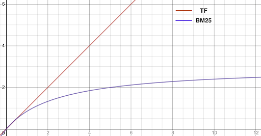
Another complication for TF is document length, especially if—as in Wikipedia—document length can vary wildly. If a document is 10,000 words long and contains cat three times, is that document more or less “about” cat than a 500-word document that contains cat twice? Various versions of length normalizations for TF try to account for this concern (as does BM25).

Math nerds can dig into more of the variants of TF–IDF on Wikipedia.

Modern problems require modern solutions

As I mentioned above, TF–IDF is quite venerable—it dates back to the 1960s! So of course modern search systems use more advanced techniques[9]—though many of these have admittedly been around (and on-wiki) for donkey’s years.

Proximity: Let us again harken back once again to our sample index statistics:

D2 has both cat and hat in it, but they are located at Word #3 and Word #45, respectively. That’s probably the same paragraph, so it’s pretty good. But D3 has them at Word #27 and Word #28—right next to each other! All other things being equal, we might want to give D2 a little boost and D3 a bigger boost in scoring.

Document structure: Query terms that are in the title of an article are probably better matches than those found in the body. Matches in the opening text of a Wikipedia article are probably more relevant than those buried in the middle of the article. Matches in the body are still better than those in the auxiliary text (image captions and the like).

Quotes: Quotes actually get overloaded in many search systems to mean search for these words as a phrase and search for these exact words. Obviously, if you only have one word in quotes—like "cats"—there’s not really a phrase there, so you are only matching the exact word. Searching for "the cats in the hats" is asking for those exact words in that exact order. On English Wikipedia, this gets zero results because searching for the exact words prevents stemmed matches to “the cat in the hat”.

A generally under-appreciated feature of on-wiki search is quotes-plus-tilde: putting a tilde after a phrase in quotes keeps the phrase order requirement, but still allows for stemming and other text processing. So "the cats in the hats"~ will in fact match “the cat in the hat”!

Query-independent features: Sometimes there are good hints about which documents are better than others that don’t depend on the query! For example, the popularity or quality of an article can be used to give those articles a boost in the rankings. (In commercial contexts, other query-independent features—like what’s on sale or overstocked, what you bought last time, or even paid ranking—could also be used to give results a boost.)

Multiple indexes: As mentioned before (in footnote 8 and in previous installments of this series), we actually use multiple indexes for on-wiki search. The “text” index uses all the text processing we’ve described along the way—tokenization, normalization, stop words, and stemming—while the “plain” field only undergoes tokenization and normalization. We can score results from each index independently and then combine them.

Multiple scores: However, when you try to combine all of the useful signals you may have about a document and a query—the TF and IDF of the query terms, where in the document the matches come from (title, opening text, auxiliary text), the popularity of the article, matches from the “text” index, matches from the “plain” index, etc., etc.—it can become very difficult to find the ideal numerical combination of all the weights and factors.

Tuning such a scoring formula can turn into a game of whack-a-mole. Every time you make a small improvement in one area, things get a little worse in another area. Many of the basic ideas that go into a score are clear—a title match is usually better than a match in the body; an exact match is usually better than a stemmed match, a more popular document is probably better than less popular document. The details, however, can be murky—is a title match twice as good as a match in the body, or three times? Is a more popular document 10% better than a less popular document, or 15%? Does popularity scale linearly, or logarithmically?

To prevent any scoring formula from getting totally out of control, you generally have to commit to a single answer to these questions. A very popular article is indeed probably best if the user’s query is just one word. However, if the user’s query is several words and also an exact title match for a much less frequently visited article, then that’s probably the best result. How do you optimize for all of that at once? And will the answer be the same for English and Russian Wikipedia? Chinese? Japanese? Hebrew? (Hint: The answer is “probably not”.)

So what do we do? Enter machine learning…

Machine learning: Machine learning is too big of a topic to even begin to properly address it here. One of the important things to know is that machine learning lets you combine a lot of potential pieces of information in a way that selects the most useful bits. It also combines them in complex and conditional ways—for example, maybe article popularity is less important when you have more search terms.

And the one of best things about machine learning is that the entire process is largely automated—if you have enough examples of the “right” answer to learn from. The automation also means that you can learn different models for different wikis and you can update your models regularly and adapt to changing patterns in the way people search.

We’ve built, tested, and deployed machine learning–based models for ranking to the 19 biggest Wikipedias (those with >1% of all search traffic): Arabic, Chinese, Dutch, English, Finnish, French, German, Hebrew, Indonesian, Italian, Japanese, Korean, Norwegian, Persian, Polish, Portuguese, Russian, Swedish, and Vietnamese.

Further reading / Homework

If you found footnote 1 and footnote 4 really interesting, read up on the “Use–mention distinction”.

I put together a video back in January of 2018, available on Commons, that covers the Bare-Bones Basics of Full-Text Search. It starts with no prerequisites, and covers tokenization and stemming, inverted indexes, basic boolean and proximity retrieval operations, TF/IDF and the vector space model of similarity, field-level indexing, and using multiple indexes, and then touches on some of the elements of scoring. If you’ve read and enjoyed all the posts in this series, then this video is a great way to reinforce the basic ideas and expand a bit into a few new areas.

Footnotes

[1] Formatting searches is hard. If I write that a user searched for “Of Cats and Hats,” does that mean they used quotes, which gives very different results? Also—independent of the quotes—was the comma included in the search string? Some people have suggested using slashes for /search strings/. This can give linguists, particularly phoneticians, mild fits, but it also causes a different kind of ambiguity if your search supports regular expressions, like /insource:/cat in the hat/i/. I prefer italics because people can’t normally type in italics in a search box—weird ??????? characters notwithstanding—but it still doesn’t solve the problem of a final period or comma!

[2] Similar to the issue of how to format queries in footnote 1, we need to be able to distinguish AND and OR the search operators from and and or the normal words.[3] Typically, we do that by capitalizing them.

[3] Speaking of normal words, and and or in common usage are not as precise as their Boolean counterparts. It’s not that hard to construct sentences where and means OR and or means AND. To wit: “I need a shirt I can wear to work or to a party.” Clearly, if someone then offered you a shirt that you could wear to a party but not to work, you would not be pleased. You are asking for a shirt that can do both (i.e., work AND party). “I have friends who play football, baseball, and soccer professionally.” You almost certainly mean you have friends who each play one of the listed sports (i.e., football OR baseball OR soccer). (Even Bo Jackson only played two of them professionally—and, chances are, you don’t know Bo.)

[4] In the old days—that is, through the 1990s—before public search engines were available on the internet and most search engine users were carefully trained lawyers, librarians, or other scholars, search operators like AND and OR where generally explicit, and queries were sometimes much more complex, with nested parentheses to make up for the lack of normalization, stemming, or thesauri. Thus, (attorney OR attorneys OR lawyer OR lawyers OR law OR laws) AND (dog OR dogs OR cat OR cats OR pet OR pets OR animal OR animals)[5] would be used, where today we expect decent results from pet lawyer—and indeed “Animal law” is the top five results on English Wikipedia as of this writing. (See also footnote 6.)

[5] Another side effect of the lack of stemming was that nouns were easier to search for than verbs—at least in English and many other European languages—because nouns often have many fewer forms. You could easily go over your query length limit trying to fit in several dozen verb forms from a Romance language, for example. Nevertheless this is one kind of query expansion that can be optionally performed when your index doesn’t use stemmed forms of words.

[6] The current (August 2019) situation with on-wiki searching and boolean operators is complex and my advice is to avoid using OR or explicit AND in your queries for now because they can give extremely unintuitive results—especially with keywords and namespaces—as the result of a low-level translation of the binary boolean formalism into an incompatible unary formalism. See more at Help:CirrusSearch/Logical operators on MediaWiki.

[7] The word iff is a weird one. Conjunctions are usually considered a closed class, so adding new ones is rare. In English it’s also generally hard to pronounce iff in a way that distinguishes it from regular if—though ifffffffffff might work. A lot of the strangeness of iff has been calqued into other languages by following a similar recipe—take the word for “if” and double one of the letters, preferably a consonant at the end of the word if one is available—giving the following pairs: Danish and Norwegian hvis/hviss, Finnish jos/joss, French si/ssi, Hebrew אםם/אם, Portuguese se/sse, Romanian dacă/ddacă, Spanish si/sii (bucking the consonant-based trend), and Swedish om/omm.

[8] As mentioned in the previous installment on indexing, on-wiki we alleviate this problem by having multiple indexes. The “text” index uses all the text processing we’ve described along the way—tokenization, normalization, stop words, and stemming—while the “plain” field only undergoes tokenization and normalization, making it possible to find “to be or not to be” and “The The”, especially as titles.

[9] Advances in search have been enabled in part by more sophisticated algorithms, but they have also been helped immeasurably by Moore’s Law. Moore’s Law roughly predicts that computing power doubles every two years; it may have started slowing down in the last few years, but it held true for decades. Thus 50 years of technological improvements have led to computers in the 2010s that are tens of millions of times faster than those of the 1960s. All that extra horsepower makes many more things possible!

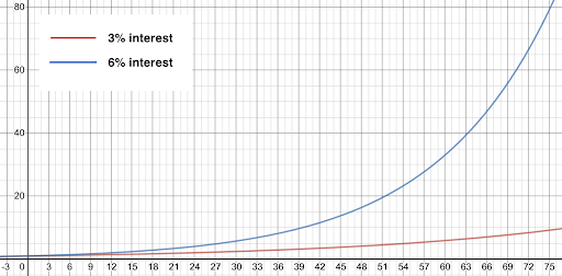
To get a little perspective on how much Moore’s Law matters, consider the following. A program that took one minute to run in 2015 might have taken almost 64 years to run on comparable hardware from 1965. So, in 1965 it would actually have been faster to wait 30 years and then run the program on new hardware in 1995, when it would have taken about 17 hours. That’s not exactly fast, but you’d only have to let it run overnight. Ten years later in 2005 and you could probably run it while you get lunch because it would take just over half an hour. If Moore’s Law does manage to hold up through 2025, the wait will be down to a couple of seconds. Exponential growth is amazing.[10]

[10] [!! MATH ALERT !!] For smaller rates of growth—i.e., well under 20% (note that Moore’s Law works out to about 41% per year, so this doesn’t apply)—you can estimate doubling time for r% growth as 72/r. It’s not accurate enough for planning the date of your retirement party, but it’s good for back-of-the-envelope calculations. 3% annual growth will double in 24 years, but in that time 6% growth will double twice—i.e., quadruple.